BEoRN: Post-processing with Merger Trees#
This notebook demonstrates how to use BEoRN with per-halo accretion rates derived from merger trees. Instead of assuming the same exponential growth rate α for all halos, we fit α individually for each halo from its mass accretion history along the main progenitor branch.
Data used: THESAN-DARK 2 — a publicly available dark-matter-only simulation (95.5 cMpc/h box, 1050³ particles, LHaloTree merger trees).
Prerequisites: Have the THESAN-DARK snapshot and merger tree data available (see FILE_ROOT in the paths cell below). The simplified tree cache is built automatically in Section 3 the first time you run the notebook.
How this tutorial is structured#
We follow the same pattern as the nbody_simulation_halos notebook: we write a custom MyMergerTreeLoader class that you can adapt for any simulation with merger trees. BEoRN ships a ready-made ThesanLoader that does exactly what MyMergerTreeLoader does below, but showing the explicit implementation makes it easy to adapt the code to other datasets (IllustrisTNG, EAGLE, Bolshoi, etc.).
The key difference from the N-body tutorial is that the loader now also reads the merger tree and returns a HaloCatalog with a per-halo alphas array.
import os
import numpy as np
from tqdm import tqdm
from pathlib import Path
import h5py
import matplotlib.pyplot as plt
import matplotlib.colors as mcolors
from matplotlib import gridspec

%matplotlib inline

import logging
logging.basicConfig(level=logging.INFO)
logger = logging.getLogger(__name__)

import beorn
from beorn.particle_mapping import map_particles_to_mesh

import matplotlib as mpl
mpl.rcParams.update({
    'font.size': 14, 'axes.labelsize': 14,
    'xtick.labelsize': 12, 'ytick.labelsize': 12,
    'legend.fontsize': 12, 'axes.titlesize': 14,
})
# ── Paths ──────────────────────────────────────────────────────────────────
# FILE_ROOT: root of the THESAN-DARK data tree.  Expected layout:
#   FILE_ROOT/output/groups_*/          ← FoF group catalogs
#   FILE_ROOT/output/snapdir_*/         ← DM particle snapshots
#   FILE_ROOT/postprocessing/offsets/   ← subhalo offset files
#   FILE_ROOT/postprocessing/trees/LHaloTree/  ← raw LHaloTree HDF5 files
# FILE_ROOT  = Path(os.environ.get("PROJECT", "input")) / "Thesan-Dark-2"
FILE_ROOT = Path("/xdisk/timeifler/yhhuang/Thesan")

# CACHE_ROOT: intermediate results (radiation profiles, tree cache)
# CACHE_ROOT = Path("cache")
CACHE_ROOT = Path("/xdisk/timeifler/yhhuang/Thesan/postprocessing/")
CACHE_ROOT.mkdir(parents=True, exist_ok=True)
CACHE_FILE = CACHE_ROOT / "Thesan-Dark-2_tree_cache.hdf5"

# OUTPUT_ROOT: where painted signal cubes are written
# OUTPUT_ROOT = Path(os.environ.get("SCRATCH", "output"))
OUTPUT_ROOT = Path("/xdisk/timeifler/yhhuang/BEoRN-v2/thesan_run/output")


# ── Snapshot to inspect ────────────────────────────────────────────────────
# Snap 49 ≈ z=7.4 in THESAN-DARK 2; adjust if your download differs.
SNAP_IDX = 49

# ── Resolution flag ────────────────────────────────────────────────────────
IS_HIGH_RES    = False  # True for THESAN-DARK 1 (2100³ particles)
PARTICLE_COUNT = 2100**3 if IS_HIGH_RES else 1050**3
import beorn

import matplotlib as mpl
mpl.rcParams.update({
    'font.size': 14, 'axes.labelsize': 14,
    'xtick.labelsize': 12, 'ytick.labelsize': 12,
    'legend.fontsize': 12, 'axes.titlesize': 14,
})
1. Set simulation and astrophysical parameters#
THESAN-DARK 2 specifics#
Box: 95.5 cMpc/h
Mass resolution: 2.96 × 10⁷ M☉ per particle → minimum resolved halo ~10⁹ M☉
Cosmology: Planck 2015 (same as IllustrisTNG)
Merger tree settings#
mass_accretion_lookback = 10: use 10 snapshots of lookback history when fitting α (Moll 2025, Fig. 3 — mean stabilises at n=10)alpha_fallback = "mean": halos not in the tree get the mean α of their snapshot (adapts with redshift)halo_mass_accretion_alpha: set to [0, 5] with 26 bins — covers the full observed range in THESAN (Moll 2025, Sec. 4.3)
parameters = beorn.structs.Parameters()

## Simulation grid — must match the THESAN data
parameters.simulation.Lbox  = 95.5    # comoving Mpc/h
parameters.simulation.Ncell = 128     # grid resolution for painting
parameters.simulation.cores = 1

## Merger tree settings
parameters.source.mass_accretion_lookback = 10   # lookback snapshots for alpha fit
parameters.source.alpha_fallback          = 'mean'  # fallback for halos not in tree

## Solver: redshift grid and alpha bins
# Covering z = 6–10 is sufficient for a single-snapshot tutorial at z≈7.4.
# Widen this range if you want to paint multiple snapshots.
parameters.solver.redshifts                 = np.arange(20.0, 5.5, -0.5)
parameters.solver.halo_mass_accretion_alpha = np.linspace(0, 5, 26)  # 25 bins, 0–5
parameters.solver.halo_mass_bin_min         = 1e8
# Upper limit must cover the most massive halo in the box at every snapshot.
# At z≈7.4 in THESAN-DARK 2 the most massive halos reach ~a few × 10¹³ M☉;
# halos above this limit fall outside all profile bins and raise an AssertionError.
parameters.solver.halo_mass_bin_max         = 5e14
parameters.solver.halo_mass_nbin            = 40

## Cosmology (Planck 2015, matching THESAN)
parameters.cosmology.Om  = 0.3089
parameters.cosmology.Ob  = 0.0486
parameters.cosmology.Ol  = 1 - 0.3089
parameters.cosmology.h0  = 0.6774

## Source model — 'boosted' model from Moll (2025) / Schaeffer et al. (2023)
parameters.source.f_st   = 0.1
parameters.source.Mp     = 2.8e10 * parameters.cosmology.h0   # pivot mass
parameters.source.g1     = 0.49
parameters.source.g2     = -0.61
parameters.source.g3     = 4
parameters.source.g4     = -4
parameters.source.halo_mass_min = 1e9

# X-ray
parameters.source.energy_cutoff_min_xray = 500
parameters.source.energy_cutoff_max_xray = 10000
parameters.source.energy_min_sed_xray    = 200
parameters.source.energy_max_sed_xray    = 10000
parameters.source.alS_xray               = 1.5
parameters.source.xray_normalisation     = 0.3 * 3.4e40

# Lyman-alpha
parameters.source.n_lyman_alpha_photons = 9690

# Ionisation
parameters.source.Nion    = 2000
parameters.source.f0_esc  = 0.2
parameters.source.pl_esc  = 0.5
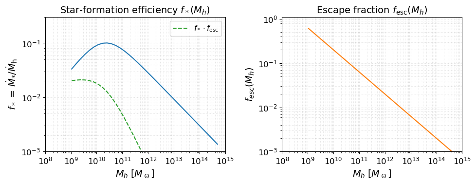
Source model visualization#
Before running anything, it is useful to inspect the astrophysical source model implied by the parameters above. The two key efficiency functions are:
Star-formation efficiency $f_*(M_h)$: fraction of accreted baryons converted into stars (double power-law with a low-mass suppression below $M_t$).
Escape fraction $f_\mathrm{esc}(M_h)$: fraction of ionising photons that escape into the IGM (power-law in halo mass).
These two functions, multiplied together and by $N_\mathrm{ion}$, set the ionising emissivity of each halo.
fig, axes = plt.subplots(1, 2, figsize=(10, 4))

beorn.plotting.draw_star_formation_rate(axes[0], parameters, color='C0')
beorn.plotting.draw_f_esc(axes[1], parameters, color='C1')

# Overlay f_star * f_esc on the left panel
Mh_grid = parameters.solver.halo_mass_bins
keep = (Mh_grid > parameters.source.halo_mass_min) & (Mh_grid <= parameters.source.halo_mass_max)
Mh_plot = Mh_grid[keep]
from beorn.astro import f_star_Halo, f_esc as f_esc_func
combined = f_star_Halo(parameters, Mh_plot) * f_esc_func(parameters, Mh_plot)
axes[0].loglog(Mh_plot, combined, color='C2', ls='--', label=r'$f_* \cdot f_\mathrm{esc}$')
axes[0].legend(fontsize=11)

axes[0].set_title(r'Star-formation efficiency $f_*(M_h)$')
axes[1].set_title(r'Escape fraction $f_\mathrm{esc}(M_h)$')

for ax in axes:
    ax.set_xlabel(r'$M_h \; [M_\odot]$')
    ax.grid(True, which='both', ls=':', alpha=0.4)
    ax.set_xlim(1e8, 1e15)
axes[0].set_ylim(1e-3, 3e-1)
axes[1].set_ylim(1e-3, 1.1)

plt.tight_layout()
plt.show()
2. Precompute radiation profiles#
Profiles are computed over a 2D grid of (halo mass, α) bins and cached. Because the α dimension is now large (25 bins vs. the default 9), the profile grid is larger — this is the expected cost of individual accretion rate treatment.
cache_handler = beorn.io.Handler(CACHE_ROOT)

solver = beorn.precomputation.RadiationProfileSolver(parameters, parameters.solver.redshifts)
# Set force_recompute=True after changing mass bin range or other profile parameters.
profiles = solver.get_or_compute_profiles(cache_handler, force_recompute=False)

print(f"Profile shape (rho_heat): {profiles.rho_heat.shape}")
print(f"  (n_r, n_mass_bins, n_alpha_bins, n_z)")
INFO:beorn.io.handler:Using persistence directory at /xdisk/timeifler/yhhuang/Thesan/postprocessing
INFO:beorn.precomputation.solver:Radiation profiles not found in cache. Launching a single computation process.
INFO:beorn.precomputation.solver:param.solver.fXh is set to constant. We will assume f_X,h = 2e-4**0.225
INFO:beorn.precomputation.solver:Computing profiles for 29 redshifts, 39 halo mass bins and 25 alpha bins.
WARNING:beorn.structs.base_struct:Field delta_b not found in RadiationProfiles. It will not be written to the HDF5 file.
WARNING:beorn.structs.base_struct:Field Grid_Temp not found in RadiationProfiles. It will not be written to the HDF5 file.
WARNING:beorn.structs.base_struct:Field Grid_xHII not found in RadiationProfiles. It will not be written to the HDF5 file.
WARNING:beorn.structs.base_struct:Field Grid_xal not found in RadiationProfiles. It will not be written to the HDF5 file.
INFO:beorn.structs.base_struct:Data written to /xdisk/timeifler/yhhuang/Thesan/postprocessing/radiation_profiles_legacy/RadiationProfiles_2ce95147.h5 (302.49 MB)
INFO:beorn.precomputation.solver:Rank 0 computed profiles and saved them to cache.
Profile shape (rho_heat): (200, 39, 25, 29)
  (n_r, n_mass_bins, n_alpha_bins, n_z)
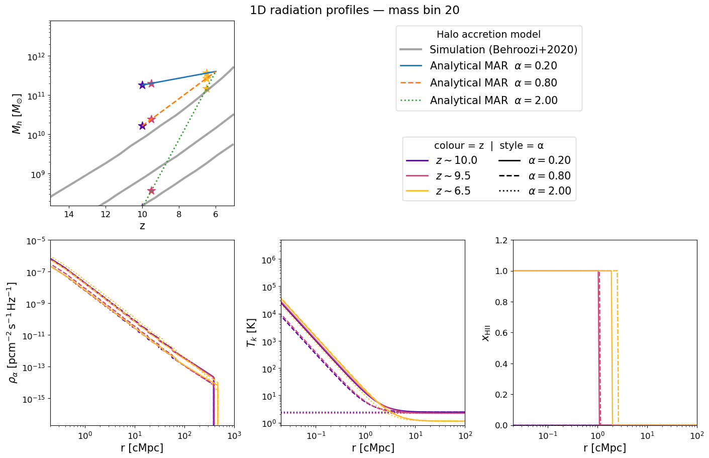
Inspecting the pre-computed 1D profiles#
The figure below mirrors Figure 2 of Schaeffer et al. 2023. Each panel corresponds to a selected halo mass bin and shows how the radial profile evolves with redshift (blue → red):
Halo mass accretion history — exponential MAR model (grey) vs. Behroozi et al. 2020 simulations (gold).
Lyman-α flux profile $\rho_\alpha(r)$ — sets the WF coupling $x_\alpha$.
Kinetic temperature profile $T_k(r)$ — driven by X-ray heating.
Ionization fraction $x_\mathrm{HII}(r)$ — sharp bubble front expanding with time.
Because we now have 25 α bins, we show three representative values — slow (α=0.3), fiducial (α=0.79), and fast (α=2.0) accretion — to illustrate how the profile shape changes with the halo accretion rate. Adjust mass_index and the lists to explore further.
mass_index = parameters.solver.halo_mass_nbin // 2
profile_redshifts = [13.0, 9.5, 6.5]
# Show three α values to highlight the impact of different accretion rates
profile_alphas = [0.3, 0.79, 2.0]

beorn.plotting.plot_1D_profiles(
    parameters,
    profiles,
    mass_index=mass_index,
    redshifts=profile_redshifts,
    alphas=profile_alphas,
    label=f"1D radiation profiles — mass bin {mass_index}",
    fontsize=15,
)
3. Prepare the simplified tree cache#
BEoRN’s merger tree loader reads a flat HDF5 cache containing four parallel arrays extracted from the raw LHaloTree files. The cache is built once and reused on subsequent runs.
The cache schema is simulation-agnostic — only these four arrays are required:
Dataset |
dtype |
Description |
|---|---|---|
|
int64 |
subhalo index within its snapshot |
|
int32 |
snapshot index |
|
float32 |
halo mass (10¹⁰ M☉/h — raw THESAN units) |
|
int64 |
flat-array index of main progenitor, or -1 |
Other simulations: Replace the reading code below with whatever reads your native format (Consistent-Trees, SubLink, etc.) while keeping the output schema identical.
if CACHE_FILE.exists():
    logger.info(f"Tree cache already exists: {CACHE_FILE} — skipping extraction.")
else:
    logger.info("Building tree cache (runs once, result cached to disk)…")

    tree_dir   = FILE_ROOT / "postprocessing" / "trees" / "LHaloTree"
    tree_files = sorted(tree_dir.glob("trees_sf1_*.hdf5"))
    tree_files = [f for f in tree_files if f.name != CACHE_FILE.name]
    if not tree_files:
        raise FileNotFoundError(f"No LHaloTree files found in {tree_dir}")

    # Read metadata from the first file's header
    with h5py.File(tree_files[0], "r") as f:
        snapshot_redshifts = f["Header"]["Redshifts"][:].tolist()
        particle_mass_1e10 = float(f["Header"].attrs["ParticleMass"])  # 10^10 M☉/h
        _h_header = float(
            f["Header"].attrs["HubbleParam"]
            if "HubbleParam" in f["Header"].attrs
            else parameters.cosmology.h0
        )
    logger.info(f"  {len(tree_files)} tree file(s), {len(snapshot_redshifts)} snapshots")

    # Auto-detect mass field (LenType preferred for THESAN-DARK because it uses
    # integer particle counts which give monotonic histories; SubhaloMassType is
    # a bound-mass estimate that can decrease due to tidal stripping).
    with h5py.File(tree_files[0], "r") as _f:
        _t      = _f["Tree0"]
        _fields = set(_t.keys())

        _mass_field = "LenType" if "LenType" in _fields else "SubhaloMassType"
        logger.info(f"Mass field: {_mass_field}")

        # Identify FoF-first-halo pointer (capitalization varies between releases)
        _fof_field = next(
            (name for name in ("FirstHaloInFOFgroup", "FirstHaloInFOFGroup",
                               "FirstHaloInFoFGroup", "FOFHalo")
             if name in _fields),
            None,
        )
        if _fof_field is None:
            raise KeyError(
                f"Cannot find a FoF-first-halo pointer in {list(_fields)}. "
                "Check the field names printed by the inspect-tree cell."
            )
        logger.info(f"FoF-central field: {_fof_field}")

    all_halo_ids, all_snap_nums, all_masses, all_main_prog, all_is_central = [], [], [], [], []
    global_offset = 0

    for tree_file in tree_files:
        with h5py.File(tree_file, "r") as f:
            tree_keys   = sorted(k for k in f.keys() if k.startswith("Tree"))
            file_offset = 0

            for tk in tree_keys:
                tree    = f[tk]
                n_local = tree["SnapNum"].shape[0]

                snap_num      = tree["SnapNum"][:].astype(np.int32)
                subhalo_index = tree["SubhaloNumber"][:].astype(np.int64)
                first_prog    = tree["FirstProgenitor"][:].astype(np.int64)

                if _mass_field == "LenType":
                    mass = tree["LenType"][:, 1].astype(np.float32) * particle_mass_1e10
                else:
                    mass = tree["SubhaloMassType"][:, 1].astype(np.float32)

                # A halo is central iff it is its own FoF-first pointer
                fof_first  = tree[_fof_field][:].astype(np.int64)
                local_idx  = np.arange(n_local, dtype=np.int64)
                is_central = (fof_first == local_idx)

                abs_offset = global_offset + file_offset
                main_prog  = np.where(
                    first_prog >= 0,
                    first_prog + abs_offset,
                    np.int64(-1),
                )

                all_halo_ids.append(subhalo_index)
                all_snap_nums.append(snap_num)
                all_masses.append(mass)
                all_main_prog.append(main_prog)
                all_is_central.append(is_central)
                file_offset += n_local

        logger.info(f"  {tree_file.name}: {file_offset:,} entries "
                    f"(cumulative {global_offset + file_offset:,})")
        global_offset += file_offset

    tree_halo_ids        = np.concatenate(all_halo_ids).astype(np.int64)
    tree_snap_nums_arr   = np.concatenate(all_snap_nums).astype(np.int32)
    tree_masses          = np.concatenate(all_masses).astype(np.float32)
    tree_main_progenitor = np.concatenate(all_main_prog).astype(np.int64)
    tree_is_central      = np.concatenate(all_is_central)

    with h5py.File(CACHE_FILE, "w") as f:
        f.attrs["format_version"]                = 2
        f.attrs["generated_by"]                  = "beorn"
        f.attrs["simulation_code"]               = "THESAN-DARK-1" if IS_HIGH_RES else "THESAN-DARK-2"
        f.attrs["is_high_res"]                   = IS_HIGH_RES
        f.attrs["hubble_param"]                  = _h_header
        f.attrs["mass_field_used"]               = _mass_field
        f.attrs["fof_field_used"]                = _fof_field
        f.attrs["n_snapshots"]                   = len(snapshot_redshifts)
        f.attrs["n_tree_files"]                  = len(tree_files)
        f.attrs["n_total_entries"]               = int(tree_halo_ids.size)
        f.attrs["particle_mass_1e10_Msol_per_h"] = particle_mass_1e10

        f.create_dataset("snapshot_redshifts",   data=np.array(snapshot_redshifts), compression="gzip")
        f.create_dataset("tree_halo_ids",        data=tree_halo_ids,        compression="gzip")
        f.create_dataset("tree_snap_num",        data=tree_snap_nums_arr,   compression="gzip")
        f.create_dataset("tree_mass",            data=tree_masses,          compression="gzip")
        f.create_dataset("tree_main_progenitor", data=tree_main_progenitor, compression="gzip")
        f.create_dataset("tree_is_central",      data=tree_is_central,      compression="gzip")

    logger.info(f"Tree cache saved → {CACHE_FILE}  ({tree_halo_ids.size:,} total entries, "
                f"{tree_is_central.sum():,} centrals)")
INFO:__main__:Tree cache already exists: /xdisk/timeifler/yhhuang/Thesan/postprocessing/Thesan-Dark-2_tree_cache.hdf5 — skipping extraction.
4. Write a merger tree loader for your simulation#
BEoRN provides MergerTreeLoader as an abstract base class for simulations with merger trees. To use your own data you subclass it and implement four methods:
Method |
What it does |
|---|---|
|
Returns a sorted array of available snapshot redshifts |
|
Reads the flat HDF5 cache and returns the four arrays |
|
Reads positions, masses, and subhalo→group mapping for one snapshot |
|
Reads the density field for one snapshot |
The base class handles the rest: walking main progenitor branches, calling vectorized_alpha_fit, applying fallback values and alpha range clamping, and assembling the HaloCatalog.
Ready-made class: BEoRN ships
ThesanLoaderwhich does exactly whatMyMergerTreeLoaderdoes below. The custom version is shown here so you can adapt it for other simulations.
class MyMergerTreeLoader(beorn.load_input_data.MergerTreeLoader):
    """Example merger tree loader for THESAN-DARK.

    Inherits tree walking, alpha fitting, fallback handling, and
    HaloCatalog assembly from MergerTreeLoader.  Only simulation-specific
    I/O is implemented here.

    Replace the four methods below with code that reads your simulation
    format.  The output schema must stay the same.
    """

    simulation_code = "THESAN-DARK"

    def __init__(self, parameters, *, cache_file=CACHE_FILE, is_high_res=IS_HIGH_RES):
        super().__init__(parameters)

        self.thesan_root    = FILE_ROOT
        self.offset_root    = self.thesan_root / "postprocessing" / "offsets"
        self.cached_tree    = Path(cache_file)
        self.particle_count = 2100**3 if is_high_res else 1050**3

        # Read snapshot redshifts and h from the HDF5 cache (format_version >= 2)
        with h5py.File(self.cached_tree, "r") as fh:
            redshifts = fh["snapshot_redshifts"][:]
            self.h    = float(fh.attrs.get("hubble_param",
                                           parameters.cosmology.h0))

        # Collect and sort snapshot directories by index
        catalogs  = sorted((self.thesan_root / "output").glob("groups_*"))
        off_files = sorted(self.offset_root.glob("offsets_*"))

        # Restrict to the solver redshift range
        z_min = parameters.solver.redshifts.min()
        z_max = parameters.solver.redshifts.max()
        idx = np.where((redshifts >= z_min) & (redshifts <= z_max))[0]

        self._snap_indices = idx                          # absolute snapshot numbers
        self._redshifts    = redshifts[idx]
        self._catalogs     = [catalogs[i]  for i in idx]
        self._offset_files = [off_files[i] for i in idx]

        logger.info(
            f"MyMergerTreeLoader: {self._redshifts.size} snapshots "
            f"z={self._redshifts.max():.2f}\u2192{self._redshifts.min():.2f}"
        )

    # ── 1. Snapshot redshifts ─────────────────────────────────────────────

    @property
    def redshifts(self):
        return self._redshifts

    # ── 2. Load the flat tree cache ───────────────────────────────────────

    def load_tree_cache(self):
        """Read the flat HDF5 cache built in Section 3."""
        with h5py.File(self.cached_tree, "r") as f:
            ids        = f["tree_halo_ids"][:]
            snaps      = f["tree_snap_num"][:]
            mass       = f["tree_mass"][:]
            prog       = f["tree_main_progenitor"][:]
            is_central = f["tree_is_central"][:]
        return ids, snaps, mass, prog, is_central

    # ── 3. Load halo positions, masses, and subhalo→group mapping ─────────

    def get_halo_information_from_catalog(self, redshift_index):
        """Read group positions and masses from THESAN group catalog HDF5 files.

        Returns:
            positions            (N, 3) float — comoving Mpc/h
            masses               (N,)   float — M☉
            subhalo_to_group_map (S,)   int   — subhalo → group index mapping
        """
        catalog_dir = self._catalogs[redshift_index]
        offset_file = self._offset_files[redshift_index]
        snap_files  = sorted(
            catalog_dir.rglob("*.hdf5"),
            key=lambda p: int(p.stem.split(".")[1]),
        )

        with h5py.File(offset_file, "r") as f:
            g_offsets = f["FileOffsets"]["Group"][:]
            s_offsets = f["FileOffsets"]["Subhalo"][:]

        n_g = int(g_offsets[-1] * 1.5)
        n_s = int(s_offsets[-1] * 1.5)

        positions = np.zeros((n_g, 3), dtype=np.float32)
        masses    = np.zeros(n_g, dtype=np.float64)
        smap      = np.zeros(n_s, dtype=np.int64)
        gp, sp    = 0, 0

        for snap_file in snap_files:
            with h5py.File(snap_file, "r") as f:
                if "GroupPos" not in f["Group"]:
                    continue
                gpos  = f["Group"]["GroupPos"][:]
                gmass = f["Group"]["GroupMass"][:]
                ge    = gp + gpos.shape[0]
                positions[gp:ge] = gpos
                masses[gp:ge]    = gmass
                gp = ge

                sub = f["Subhalo"]["SubhaloGrNr"][:]
                se  = sp + sub.shape[0]
                smap[sp:se] = sub
                sp = se

        positions = positions[:gp]
        masses    = masses[:gp]
        smap      = smap[:sp]

        # Unit conversions: kpc/h → Mpc/h,  10^10 M☉/h → M☉
        positions /= (1e3 * self.h)
        masses    *= 1e10 / self.h
        return positions, masses, smap

    # ── 4. Load density field (from raw particle snapshots) ───────────────

    def load_density_field(self, redshift_index):
        """Paint DM particles onto a grid and return overdensity δ = ρ/⟨ρ⟩ - 1.

        Uses map_particles_to_mesh with backend='numpy' (no extra dependencies).
        Other backends: 'numba', 'pylians', 'torch', 'jax'.
        """
        snap_idx   = int(self._snap_indices[redshift_index])  # absolute snapshot number
        snap_dir   = self.thesan_root / "output" / f"snapdir_{snap_idx:03d}"
        snap_files = sorted(snap_dir.glob("snap_*.hdf5"))

        with h5py.File(snap_files[0], "r") as f:
            box_kpc = float(f["Header"].attrs["BoxSize"])  # kpc/h

        box_mpc = box_kpc * 1e-3 / self.h
        N       = self.parameters.simulation.Ncell
        mesh    = np.zeros((N, N, N), dtype=np.float32)

        for snap in snap_files:
            with h5py.File(snap, "r") as f:
                pos = f["PartType1"]["Coordinates"][:].astype(np.float32)
            pos *= 1e-3 / self.h  # kpc/h → Mpc
            map_particles_to_mesh(mesh, box_mpc, pos,
                                  mass_assignment="CIC", backend="numpy")

        mean = mesh.mean()
        if mean > 0:
            mesh = mesh / mean - 1.0
        return mesh
Instantiate the loader#
Shortcut: Replace
MyMergerTreeLoaderwithbeorn.load_input_data.ThesanLoaderto use the production-ready version shipped with BEoRN — it is identical to the class above.
loader = MyMergerTreeLoader(parameters)

# Production-ready alternative (identical result):
# loader = beorn.load_input_data.ThesanLoader(parameters)

print(f"Loaded {loader.redshifts.size} snapshots: "
      f"z = {loader.redshifts.max():.2f} → {loader.redshifts.min():.2f}")
INFO:__main__:MyMergerTreeLoader: 69 snapshots z=19.22→6.04
Loaded 69 snapshots: z = 19.22 → 6.04
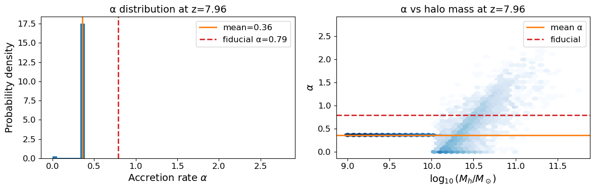
5. Inspect the halo catalog and alpha distribution#
Unlike the N-body tutorial, each halo now has an individual accretion rate α. We inspect the α distribution and compare it with the mean and the fiducial fixed value of 0.79.
# Pick a redshift to inspect — choose one with many halos
z_target = 8.0
z_index  = int(np.argmin(np.abs(loader.redshifts - z_target)))
z_actual = float(loader.redshifts[z_index])
print(f"Inspecting snapshot z={z_actual:.3f} (index {z_index})")

catalog = loader.load_halo_catalog(z_index)
print(f"Halos: {catalog.masses.size:,}")
print(f"α — mean: {catalog.alphas.mean():.2f}  "
      f"std: {catalog.alphas.std():.2f}  "
      f"min: {catalog.alphas.min():.2f}  "
      f"max: {catalog.alphas.max():.2f}")
Inspecting snapshot z=7.961 (index 15)
Halos: 315,788
α — mean: 0.36  std: 0.07  min: -0.00  max: 2.78
fig, axes = plt.subplots(1, 2, figsize=(12, 4))

# α distribution
axes[0].hist(catalog.alphas, bins=50, density=True, color='C0')
axes[0].axvline(catalog.alphas.mean(), color='C1', lw=2, label=f'mean={catalog.alphas.mean():.2f}')
axes[0].axvline(0.79, color='C3', lw=2, ls='--', label='fiducial α=0.79')
axes[0].set_xlabel(r'Accretion rate $\alpha$')
axes[0].set_ylabel('Probability density')
axes[0].set_title(f'α distribution at z={z_actual:.2f}')
axes[0].legend()

# α vs halo mass scatter
log_mass = np.log10(catalog.masses)
axes[1].hexbin(log_mass, catalog.alphas, gridsize=40, cmap='Blues',
               bins='log', mincnt=1)
axes[1].axhline(catalog.alphas.mean(), color='C1', lw=2, label='mean α')
axes[1].axhline(0.79, color='C3', lw=2, ls='--', label='fiducial')
axes[1].set_xlabel(r'$\log_{10}(M_h / M_\odot)$')
axes[1].set_ylabel(r'$\alpha$')
axes[1].set_title(f'α vs halo mass at z={z_actual:.2f}')
axes[1].legend()

plt.tight_layout()
plt.show()
6. Paint the 3D signal maps#
output_handler = beorn.io.Handler(OUTPUT_ROOT, input_tag=loader.input_tag)

# Find the redshift of snapshot SNAP_IDX so we can pass it to redshift_subset.
# The loader only exposes redshifts within parameters.solver.redshifts, so
# we pick the closest one.
with h5py.File(CACHE_FILE, 'r') as _f:
    _all_z = _f['snapshot_redshifts'][:]
z_snap = float(_all_z[SNAP_IDX])
print(f'Painting snapshot {SNAP_IDX}  (z = {z_snap:.3f})')

p = beorn.painting.PaintingCoordinator(
    parameters,
    loader=loader,
    output_handler=output_handler,
    force_recompute=False,
)

# redshift_subset restricts painting to a single snapshot.
# Remove the argument (or pass the full loader.redshifts list) to paint all.
multi_z_quantities = p.paint_full(profiles, redshift_subset=[z_snap])
INFO:beorn.io.handler:Using persistence directory at /xdisk/timeifler/yhhuang/BEoRN-v2/thesan_run/output
INFO:beorn.painting.coordinator:redshift_subset: painting 1 of 42 available snapshot(s) (42 have halo catalogs).
INFO:beorn.painting.coordinator:============================================================
BEoRN model summary
============================================================
  Cosmology   : Om=0.3089, Ob=0.0486, h0=0.6774, sigma_8=0.83
  Grid        : Ncell=128, Lbox=95.5 Mpc/h
  Profile z   : z=10.0 -> 6.0 (9 steps)
  1D RT bins  : 1.0e+08 - 5.0e+14 Msun at z=6.0 (40 bins, traced back via exp. accretion)
  Source      : f_st=0.1, Nion=2000, f0_esc=0.2
  X-ray       : norm=1.02e+40, E=[500, 10000] eV
  Lyman-alpha : n_phot=9690, star-forming above 1.0e+09 Msun
  Beorn hash  : 68e64701
============================================================
INFO:beorn.painting.coordinator:Painting profiles onto grid for 1 of 42 redshift snapshots. Using 1 processes on a single node.
Painting snapshot 49 (z = 7.430)
INFO:beorn.painting.coordinator:Painting 395643 halos at zgrid=7.50 (z_index=21).
INFO:beorn.painting.coordinator:Profile painting took 0:01:22.824799.
INFO:beorn.painting.spread:Universe not fully ionized : xHII is 0.2304.
INFO:beorn.painting.coordinator:Redistributing excess photons from the overlapping regions took 0:00:20.361469.
INFO:beorn.painting.coordinator:Postprocessing of the grids took 0:00:00.482532.
INFO:beorn.painting.coordinator:Current snapshot took 0:09:18.056391.
INFO:beorn.structs.base_struct:Data written to /xdisk/timeifler/yhhuang/BEoRN-v2/thesan_run/output/igm_data_thesan_dark_N128_L95_80daf882_68e64701/CoevalCube_z7.500.h5 (56.02 MB)
INFO:beorn.painting.coordinator:Painting of 1 snapshots done.
INFO:beorn.structs.temporal_cube:Opened 1 snapshots from /xdisk/timeifler/yhhuang/BEoRN-v2/thesan_run/output/igm_data_thesan_dark_N128_L95_80daf882_68e64701 (grid data is lazy — slices load on demand).
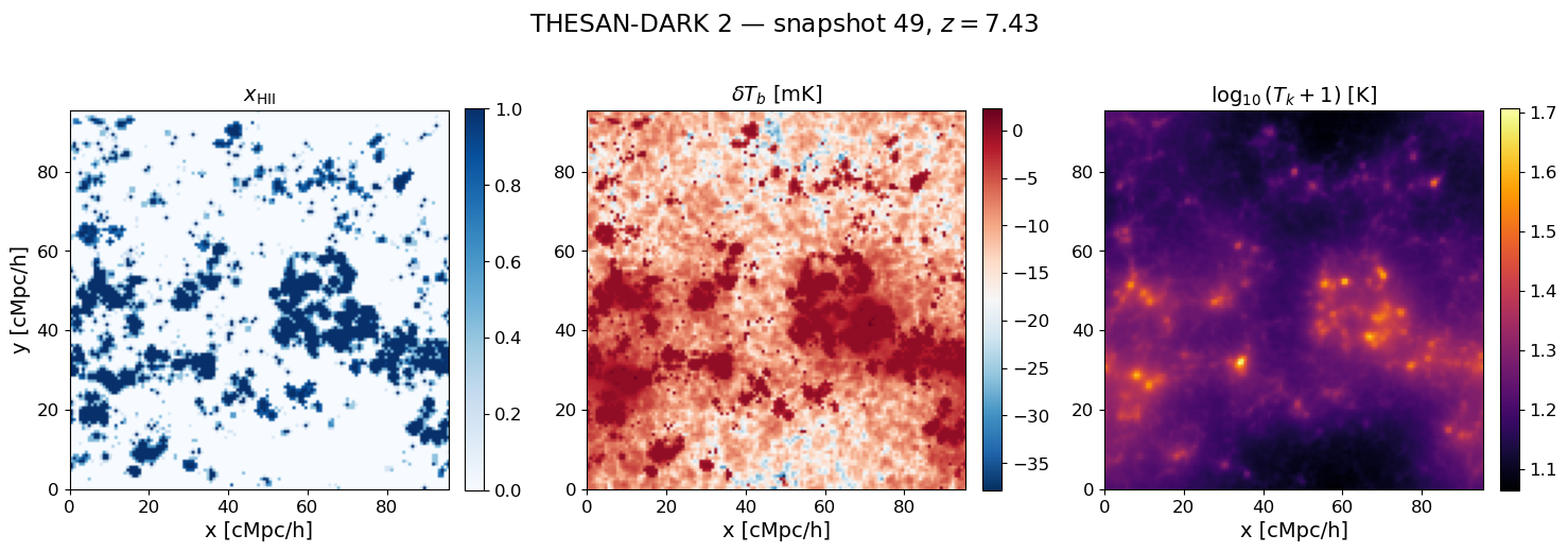
7. Visualise the 3D maps at a single redshift#
snap      = multi_z_quantities.snapshot(z_snap)
xHII_grid = snap.Grid_xHII[:]
dTb_grid  = snap.Grid_dTb
Tk_grid   = snap.Grid_Temp[:]

mid  = xHII_grid.shape[1] // 2
Lbox = parameters.simulation.Lbox
ext  = [0, Lbox, 0, Lbox]

fig, axes = plt.subplots(1, 3, figsize=(15, 5))
im0 = axes[0].imshow(xHII_grid[:, mid, :], origin='lower', extent=ext, cmap='Blues', vmin=0, vmax=1)
im1 = axes[1].imshow(dTb_grid[:, mid, :], origin='lower', extent=ext, cmap='RdBu_r')
im2 = axes[2].imshow(np.log10(Tk_grid[:, mid, :] + 1), origin='lower', extent=ext, cmap='inferno')

for ax, im, label in zip(axes,
                          [im0, im1, im2],
                          [r'$x_{\rm HII}$', r'$\delta T_b$ [mK]', r'$\log_{10}(T_k + 1)$ [K]']):
    plt.colorbar(im, ax=ax, fraction=0.046, pad=0.04)
    ax.set_xlabel('x [cMpc/h]')
    ax.set_title(label)

axes[0].set_ylabel('y [cMpc/h]')
fig.suptitle(rf'THESAN-DARK 2 — snapshot {SNAP_IDX}, $z = {z_snap:.2f}$', y=1.01)
plt.tight_layout()
plt.show()
8. Global history and power spectra#
output_handler = beorn.io.Handler(OUTPUT_ROOT, input_tag=loader.input_tag)

with h5py.File(CACHE_FILE, 'r') as _f:
    _all_z = _f['snapshot_redshifts'][:]

z_target = np.arange(19, 5.5, -1.0)
idx = np.argmin(np.abs(_all_z[:,None] - z_target[None, :]), axis=0)

redshift_subset = _all_z[idx]
print(redshift_subset)
INFO:beorn.io.handler:Using persistence directory at /xdisk/timeifler/yhhuang/BEoRN-v2/thesan_run/output
[19.21861267 17.80301476 17.16749954 16.09026337 15.20020962 13.95128345
 13.0111227  11.88165379 10.97974968 10.0561924   9.01077461  7.96091413
  7.02115583  5.99048901]
parameters.simulation.cores = 6
p = beorn.painting.PaintingCoordinator(
    parameters,
    loader=loader,
    output_handler=output_handler,
    force_recompute=False,
)

multi_z_quantities = p.paint_full(profiles, redshift_subset=redshift_subset)
INFO:beorn.painting.coordinator:redshift_subset: painting 14 of 69 available snapshot(s) (69 have halo catalogs).
INFO:beorn.painting.coordinator:============================================================
BEoRN model summary
============================================================
  Cosmology   : Om=0.3089, Ob=0.0486, h0=0.6774, sigma_8=0.83
  Grid        : Ncell=128, Lbox=95.5 Mpc/h
  Profile z   : z=20.0 -> 6.0 (29 steps)
  1D RT bins  : 1.0e+08 - 5.0e+14 Msun at z=6.0 (40 bins, traced back via exp. accretion)
  Source      : f_st=0.1, Nion=2000, f0_esc=0.2
  X-ray       : norm=1.02e+40, E=[500, 10000] eV
  Lyman-alpha : n_phot=9690, star-forming above 1.0e+09 Msun
  Beorn hash  : c9d8299b
============================================================
INFO:beorn.painting.coordinator:Painting profiles onto grid for 14 of 69 redshift snapshots. Using 6 processes on a single node.
WARNING:beorn.load_input_data.merger_tree_base:Only 1 lookback snapshots available (requested 10); returning near-zero fallback alphas for early snapshot.
INFO:beorn.painting.coordinator:Painting 15 halos at zgrid=19.00 (z_index=0).
INFO:beorn.painting.coordinator:Profile painting took 0:00:01.220958.
INFO:beorn.painting.spread:Universe not fully ionized : xHII is 0.0.
INFO:beorn.painting.coordinator:Redistributing excess photons from the overlapping regions took 0:00:00.080783.
INFO:beorn.painting.coordinator:Postprocessing of the grids took 0:00:00.474596.
INFO:beorn.painting.coordinator:Current snapshot took 0:07:09.070098.
INFO:beorn.structs.base_struct:Data written to /xdisk/timeifler/yhhuang/BEoRN-v2/thesan_run/output/igm_data_thesan_dark_N128_L95_80daf882_c9d8299b/CoevalCube_z19.000.h5 (56.02 MB)
WARNING:beorn.load_input_data.merger_tree_base:Only 3 lookback snapshots available (requested 10); returning near-zero fallback alphas for early snapshot.
INFO:beorn.painting.coordinator:Painting 115 halos at zgrid=18.00 (z_index=2).
INFO:beorn.painting.coordinator:Profile painting took 0:00:01.244595.
INFO:beorn.painting.spread:Universe not fully ionized : xHII is 0.0.
INFO:beorn.painting.coordinator:Redistributing excess photons from the overlapping regions took 0:00:00.077114.
INFO:beorn.painting.coordinator:Postprocessing of the grids took 0:00:00.492617.
INFO:beorn.painting.coordinator:Current snapshot took 0:06:57.498483.
INFO:beorn.structs.base_struct:Data written to /xdisk/timeifler/yhhuang/BEoRN-v2/thesan_run/output/igm_data_thesan_dark_N128_L95_80daf882_c9d8299b/CoevalCube_z18.000.h5 (56.02 MB)
WARNING:beorn.load_input_data.merger_tree_base:Only 4 lookback snapshots available (requested 10); returning near-zero fallback alphas for early snapshot.
INFO:beorn.painting.coordinator:Painting 228 halos at zgrid=17.00 (z_index=3).
INFO:beorn.painting.coordinator:Profile painting took 0:00:01.307962.
INFO:beorn.painting.spread:Universe not fully ionized : xHII is 0.0.
INFO:beorn.painting.coordinator:Redistributing excess photons from the overlapping regions took 0:00:00.084021.
INFO:beorn.painting.coordinator:Postprocessing of the grids took 0:00:00.491254.
INFO:beorn.painting.coordinator:Current snapshot took 0:06:53.397882.
INFO:beorn.structs.base_struct:Data written to /xdisk/timeifler/yhhuang/BEoRN-v2/thesan_run/output/igm_data_thesan_dark_N128_L95_80daf882_c9d8299b/CoevalCube_z17.000.h5 (56.02 MB)
WARNING:beorn.load_input_data.merger_tree_base:Only 6 lookback snapshots available (requested 10); returning near-zero fallback alphas for early snapshot.
INFO:beorn.painting.coordinator:Painting 735 halos at zgrid=16.00 (z_index=5).
INFO:beorn.painting.coordinator:Profile painting took 0:00:01.447471.
INFO:beorn.painting.spread:Universe not fully ionized : xHII is 0.0.
INFO:beorn.painting.coordinator:Redistributing excess photons from the overlapping regions took 0:00:00.078225.
INFO:beorn.painting.coordinator:Postprocessing of the grids took 0:00:00.487156.
INFO:beorn.painting.coordinator:Current snapshot took 0:07:12.717644.
INFO:beorn.structs.base_struct:Data written to /xdisk/timeifler/yhhuang/BEoRN-v2/thesan_run/output/igm_data_thesan_dark_N128_L95_80daf882_c9d8299b/CoevalCube_z16.000.h5 (56.02 MB)
WARNING:beorn.load_input_data.merger_tree_base:Only 8 lookback snapshots available (requested 10); returning near-zero fallback alphas for early snapshot.
INFO:beorn.painting.coordinator:Painting 1808 halos at zgrid=15.00 (z_index=7).
INFO:beorn.painting.coordinator:Profile painting took 0:00:01.498850.
INFO:beorn.painting.spread:Universe not fully ionized : xHII is 0.0.
INFO:beorn.painting.coordinator:Redistributing excess photons from the overlapping regions took 0:00:00.080936.
INFO:beorn.painting.coordinator:Postprocessing of the grids took 0:00:00.490241.
INFO:beorn.painting.coordinator:Current snapshot took 0:07:06.096646.
INFO:beorn.structs.base_struct:Data written to /xdisk/timeifler/yhhuang/BEoRN-v2/thesan_run/output/igm_data_thesan_dark_N128_L95_80daf882_c9d8299b/CoevalCube_z15.000.h5 (56.02 MB)
INFO:beorn.painting.coordinator:Painting 5813 halos at zgrid=14.00 (z_index=10).
INFO:beorn.painting.coordinator:Profile painting took 0:00:03.211022.
INFO:beorn.painting.spread:Universe not fully ionized : xHII is 0.0002.
INFO:beorn.painting.coordinator:Redistributing excess photons from the overlapping regions took 0:00:00.654680.
INFO:beorn.painting.coordinator:Postprocessing of the grids took 0:00:00.500342.
INFO:beorn.painting.coordinator:Current snapshot took 0:07:09.719431.
INFO:beorn.structs.base_struct:Data written to /xdisk/timeifler/yhhuang/BEoRN-v2/thesan_run/output/igm_data_thesan_dark_N128_L95_80daf882_c9d8299b/CoevalCube_z14.000.h5 (56.02 MB)
INFO:beorn.painting.coordinator:Painting 13063 halos at zgrid=13.00 (z_index=13).
INFO:beorn.painting.coordinator:Profile painting took 0:00:03.832413.
INFO:beorn.painting.spread:Universe not fully ionized : xHII is 0.001.
INFO:beorn.painting.coordinator:Redistributing excess photons from the overlapping regions took 0:00:00.692453.
INFO:beorn.painting.coordinator:Postprocessing of the grids took 0:00:00.502861.
INFO:beorn.painting.coordinator:Current snapshot took 0:07:12.146626.
INFO:beorn.structs.base_struct:Data written to /xdisk/timeifler/yhhuang/BEoRN-v2/thesan_run/output/igm_data_thesan_dark_N128_L95_80daf882_c9d8299b/CoevalCube_z13.000.h5 (56.02 MB)
INFO:beorn.painting.coordinator:Painting 31234 halos at zgrid=12.00 (z_index=17).
INFO:beorn.painting.coordinator:Profile painting took 0:00:06.182874.
INFO:beorn.painting.spread:Universe not fully ionized : xHII is 0.004.
INFO:beorn.painting.coordinator:Redistributing excess photons from the overlapping regions took 0:00:01.043303.
INFO:beorn.painting.coordinator:Postprocessing of the grids took 0:00:00.500313.
INFO:beorn.painting.coordinator:Current snapshot took 0:07:03.229090.
INFO:beorn.structs.base_struct:Data written to /xdisk/timeifler/yhhuang/BEoRN-v2/thesan_run/output/igm_data_thesan_dark_N128_L95_80daf882_c9d8299b/CoevalCube_z12.000.h5 (56.02 MB)
INFO:beorn.painting.coordinator:Painting 58988 halos at zgrid=11.00 (z_index=21).
INFO:beorn.painting.coordinator:Profile painting took 0:00:07.762940.
INFO:beorn.painting.spread:Universe not fully ionized : xHII is 0.0114.
INFO:beorn.painting.coordinator:Redistributing excess photons from the overlapping regions took 0:00:02.315099.
INFO:beorn.painting.coordinator:Postprocessing of the grids took 0:00:00.488048.
INFO:beorn.painting.coordinator:Current snapshot took 0:07:00.131839.
INFO:beorn.structs.base_struct:Data written to /xdisk/timeifler/yhhuang/BEoRN-v2/thesan_run/output/igm_data_thesan_dark_N128_L95_80daf882_c9d8299b/CoevalCube_z11.000.h5 (56.02 MB)
INFO:beorn.painting.coordinator:Painting 105861 halos at zgrid=10.00 (z_index=26).
INFO:beorn.painting.coordinator:Profile painting took 0:00:10.277467.
INFO:beorn.painting.spread:Universe not fully ionized : xHII is 0.031.
INFO:beorn.painting.coordinator:Redistributing excess photons from the overlapping regions took 0:00:06.785691.
INFO:beorn.painting.coordinator:Postprocessing of the grids took 0:00:00.489870.
INFO:beorn.painting.coordinator:Current snapshot took 0:07:12.619836.
INFO:beorn.structs.base_struct:Data written to /xdisk/timeifler/yhhuang/BEoRN-v2/thesan_run/output/igm_data_thesan_dark_N128_L95_80daf882_c9d8299b/CoevalCube_z10.000.h5 (56.02 MB)
INFO:beorn.painting.coordinator:Painting 189731 halos at zgrid=9.00 (z_index=33).
INFO:beorn.painting.coordinator:Profile painting took 0:00:13.283171.
INFO:beorn.painting.spread:Universe not fully ionized : xHII is 0.0756.
INFO:beorn.painting.coordinator:Redistributing excess photons from the overlapping regions took 0:00:13.236556.
INFO:beorn.painting.coordinator:Postprocessing of the grids took 0:00:00.482361.
INFO:beorn.painting.coordinator:Current snapshot took 0:07:16.445870.
INFO:beorn.structs.base_struct:Data written to /xdisk/timeifler/yhhuang/BEoRN-v2/thesan_run/output/igm_data_thesan_dark_N128_L95_80daf882_c9d8299b/CoevalCube_z9.000.h5 (56.02 MB)
INFO:beorn.painting.coordinator:Painting 315788 halos at zgrid=8.00 (z_index=42).
INFO:beorn.painting.coordinator:Profile painting took 0:00:19.486022.
INFO:beorn.painting.spread:Universe not fully ionized : xHII is 0.1638.
INFO:beorn.painting.coordinator:Redistributing excess photons from the overlapping regions took 0:00:21.341518.
INFO:beorn.painting.coordinator:Postprocessing of the grids took 0:00:00.476387.
INFO:beorn.painting.coordinator:Current snapshot took 0:07:36.149149.
INFO:beorn.structs.base_struct:Data written to /xdisk/timeifler/yhhuang/BEoRN-v2/thesan_run/output/igm_data_thesan_dark_N128_L95_80daf882_c9d8299b/CoevalCube_z8.000.h5 (56.02 MB)
INFO:beorn.painting.coordinator:Painting 462562 halos at zgrid=7.00 (z_index=53).
INFO:beorn.painting.coordinator:Profile painting took 0:00:26.743557.
INFO:beorn.painting.spread:Universe not fully ionized : xHII is 0.3037.
INFO:beorn.painting.coordinator:Redistributing excess photons from the overlapping regions took 0:00:16.591647.
INFO:beorn.painting.coordinator:Postprocessing of the grids took 0:00:00.467197.
INFO:beorn.painting.coordinator:Current snapshot took 0:07:38.218191.
INFO:beorn.structs.base_struct:Data written to /xdisk/timeifler/yhhuang/BEoRN-v2/thesan_run/output/igm_data_thesan_dark_N128_L95_80daf882_c9d8299b/CoevalCube_z7.000.h5 (56.02 MB)
INFO:beorn.painting.coordinator:Painting 641692 halos at zgrid=6.00 (z_index=68).
INFO:beorn.painting.coordinator:Profile painting took 0:00:35.778157.
INFO:beorn.painting.spread:Universe not fully ionized : xHII is 0.5249.
INFO:beorn.painting.coordinator:Redistributing excess photons from the overlapping regions took 0:00:10.709348.
INFO:beorn.painting.coordinator:Postprocessing of the grids took 0:00:00.434150.
INFO:beorn.painting.coordinator:Current snapshot took 0:07:43.170436.
INFO:beorn.structs.base_struct:Data written to /xdisk/timeifler/yhhuang/BEoRN-v2/thesan_run/output/igm_data_thesan_dark_N128_L95_80daf882_c9d8299b/CoevalCube_z6.000.h5 (56.02 MB)
INFO:beorn.painting.coordinator:Painting of 14 snapshots done.
INFO:beorn.structs.temporal_cube:Opened 14 snapshots from /xdisk/timeifler/yhhuang/BEoRN-v2/thesan_run/output/igm_data_thesan_dark_N128_L95_80daf882_c9d8299b (grid data is lazy — slices load on demand).
fig = plt.figure(constrained_layout=True, figsize=(18, 6))
gs = gridspec.GridSpec(2, 3, figure=fig)
ax1 = fig.add_subplot(gs[:, 0])
ax2 = fig.add_subplot(gs[0, 1])
ax3 = fig.add_subplot(gs[1, 1], sharex=ax2)
ax4 = fig.add_subplot(gs[:, 2])
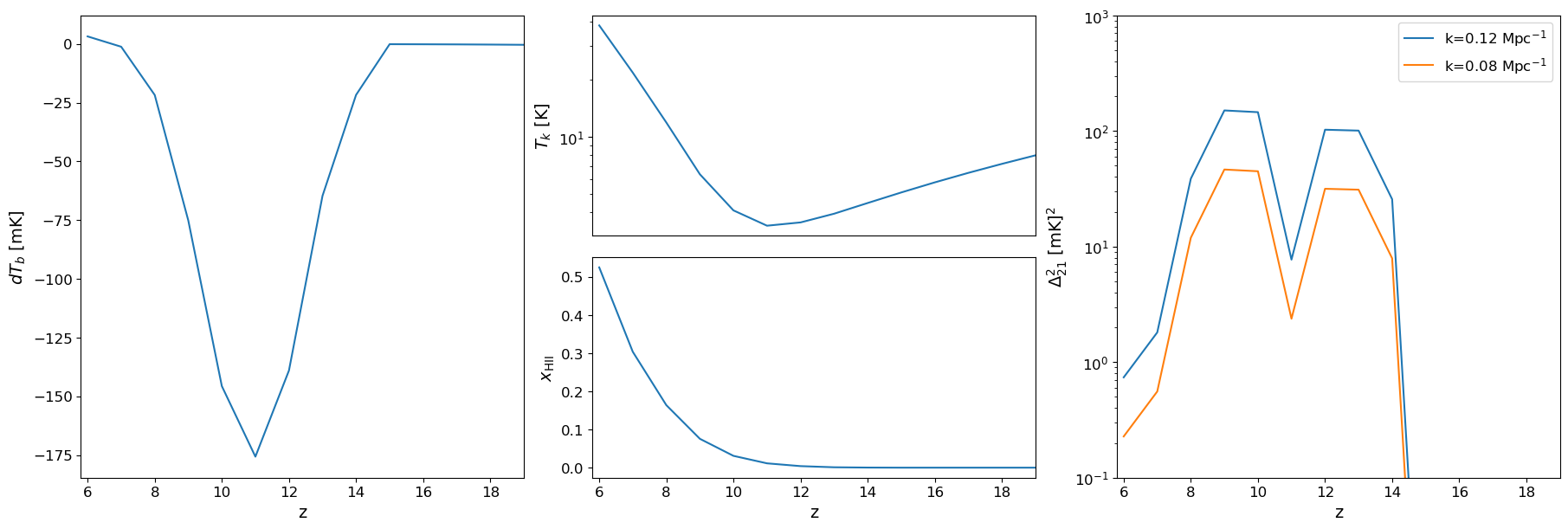
beorn.plotting.draw_dTb_signal(ax1, multi_z_quantities, label='individual α (merger tree)')
beorn.plotting.draw_Temp_signal(ax2, multi_z_quantities)
beorn.plotting.draw_xHII_signal(ax3, multi_z_quantities)
kplot1 = beorn.plotting.draw_dTb_power_spectrum_of_z(
ax4, multi_z_quantities, parameters, k_value=0.12)
kplot2 = beorn.plotting.draw_dTb_power_spectrum_of_z(
ax4, multi_z_quantities, parameters, k_value=0.05)
ax4.plot([], [], color='C0', label=f'k={kplot1:.2f} Mpc$^{{-1}}$')
ax4.plot([], [], color='C1', label=f'k={kplot2:.2f} Mpc$^{{-1}}$')
ax4.legend(loc=0)
ax2.axes.get_xaxis().set_visible(False)
fig.show()
k=0.12 Mpc$^{-1}$
k=0.08 Mpc$^{-1}$
9. Compare with fixed α = 0.79 (optional)#
To reproduce the comparison from Moll (2025) Fig. 6, run the painting a second time with a fixed α for all halos. This requires new profiles (different alpha bins) and a second output directory.
The key difference expected:
Heating delayed by Δz ≈ 0.5 with individual α (mean α < 0.79 in THESAN)
Absorption trough shifted to later times, shallower
Ionization history largely unchanged
# parameters_fixed = beorn.structs.Parameters()   # copy and adjust
# parameters_fixed.solver.halo_mass_accretion_alpha = np.array([0.7, 0.79, 0.9])  # single bin around 0.79
# ... run profiles + painting in OUTPUT_ROOT/fixed_alpha/ ...